
\[\begin{align} \dot{x}&=Ax\\ x &\in \mathbb{R}^n\\ A &\in \mathbb{R}^{n \times n}\\ x(0) &= x_0 \in \mathbb{R}^n \text{ (initial condition) }\\ \end{align}\]
Recall:
Motivated by 1 and 2, define the matrix exponential:
\[e^A := I + A + \frac{A^2}{2!} + ...\]
\[\begin{align} A &= \begin{bmatrix}0 & 0 \\ 0 & 0\end{bmatrix}\\ \Rightarrow e^A &= I + 0 + 0 + ...\\ &= \begin{bmatrix}1 & 0 \\ 0 & 1\end{bmatrix}\\ \end{align}\]
\[\begin{align} A &= \begin{bmatrix}1 & 0 \\ 0 & 2\end{bmatrix}\\ \text{For a diagonal matrix:}\\ A^k &= \begin{bmatrix}1^k & 0 \\ 0 & 2^k\end{bmatrix}\\ \Rightarrow e^A &= I + \begin{bmatrix}1 & 0 \\ 0 & 2\end{bmatrix} + \begin{bmatrix}1^2 & 0 \\ 0 & 2^2\end{bmatrix} + ...\\ &= \begin{bmatrix}e^1 & 0 \\ 0 & e^2\end{bmatrix}\\ \end{align}\]
\[
A = \begin{bmatrix}0 & 1 & 0 \\ 0 & 0 & 1 \\ 0 & 0 & 0\end{bmatrix}\\
\]
Check that \(A^3=0\) (i.e. \(A\) is nilpotent).
\[
e^A = I + A + \frac{A^2}{2} = \begin{bmatrix}1 & 1 & \frac{1}{2} \\ 0 & 1 & 1 \\ 0 & 0 & 1\end{bmatrix}\\
\]
Replace \(A\) with \(tA\) to get a function of time:
\[e^{At} = I + tA + \frac{t^2A^2}{2!} + ...\]
Theorem: The unique solution to \(\dot{x}=Ax, \quad x(0)=x_0\) is \(x(t)=e^{tA}x_0\).
Take the Laplace transform of \(\dot{x}=Ax\) without assuming \(x(0)=0\):
\[\begin{align}
sX(s) - x(0) &= AX(s)\\
X(s) &= (sI-A)^{-1} x(0)\\
\end{align}\]
Conclusion: \(e^{At}\) and \((sI-A)^{-1}\) are Laplace transform pairs.
\[\begin{align} A &= \begin{bmatrix}0&1&0\\0&0&1\\0&0&0\end{bmatrix}\\ sI-A &= \begin{bmatrix}s&-1&0\\0&s&-1\\0&0&s\end{bmatrix}\\ (sI-A)^{-1} &= \frac{\text{adj}(sI-A)}{\det(sI-A)}\\ &= \frac{1}{s^3} \begin{bmatrix}s^2&s&1\\0&s^2&s\\0&0&s^2\end{bmatrix}\\ e^{tA} &= \mathcal{L}^{-1} \left\{ (sI-A)^{-1} \right\}\\ &= \begin{bmatrix}1&t&\frac{t^2}{2}\\0&1&t\\0&0&1\end{bmatrix}, \quad t \ge 0\\ \end{align}\]
The solution of \(\dot{x}=Ax+Bu\), \(y=Cx+Du\), \(x(0)=x_0\) is:
\[x(t) = \underbrace{e^{At}x_0}_\text{initial state response} + \underbrace{\int_0^t e^{A(t-\tau)} Bu(\tau)d\tau}_\text{forced response}\]
\[Y(t)=Cx(t)+Du(t)\]
In SISO (single-input-single-output) special case where \(x(0)=0\), we get the familiar result:
\[\begin{align}
y(t)&=(g * u)(t) = \int_0^t g(t-\tau)u(\tau)d\tau\\
g(t)&=Ce^{At}B 1(t) + D\delta(t)
\end{align}\]
Where \(1(t)\) is the unit step function and \(\delta(t)\) is the unit impulse.
The system \(\dot{x}=Ax\) is asymptotically stable if \(x(t) \rightarrow 0\) for any initial condition.
\(e^{At} \rightarrow 0\) if and only if all the eigenvalues of \(A\) have a negative real part.
\[\begin{align} M\ddot{q}&=u-Kq \quad \text{(mass-spring)}\\ x &= \begin{bmatrix}x_1\\x_2\end{bmatrix} := \begin{bmatrix}q\\\dot{q}\end{bmatrix}\\ \dot{x} &= \begin{bmatrix}0&1\\\frac{-k}{M}&0\end{bmatrix}x + \begin{bmatrix}0\\\frac{1}{M}\end{bmatrix}u\\ \\ \text{Using } M=1, k=4:\\ e^{At} &= \begin{bmatrix}\cos 2t&\frac{1}{2}\sin 2t\\-2\sin 2t & \cos 2t\end{bmatrix}\\ \end{align}\]
Since \(e^{At}\) does not approach 0 as \(t\) grows large, the system is not asymptotically stable.
Let's double-check this using the eigenvalues. Solve for \(s\) such that \(\det(sI-A)=0\).
\[\begin{align}
A &= \begin{bmatrix}0 & 1 \\ -4 & 0 \end{bmatrix}\\
\det \begin{bmatrix}s & -1 \\ 4 & s\end{bmatrix} &= 0\\
s^2 + 4 &= 0\\
s &= \pm 2j
\end{align}\]
The system is therefore not asymptotically stable since it has at least one eigenvalue (in this case, it has two) with a non-negative real part.
If we introduce friction:
\[\begin{align}
\ddot{q} &= u-4q-\dot{q}
\end{align}\]
Check that it is asymptotically stable (it should be)
\[ Y(s)=G(s)U(s) \quad \text{or} \quad y(t)=(g*u)(t), g(t)=\mathcal{L}^{-1}\left\{G(s)\right\}\\ \]
A signal \(u(t)\) is bounded if there exists a constant \(b\) such that, for all \(t \ge 0\), \(|u(t)| \le b\).
For example, \(\sin t\) is bounded by \(b=1\).
If \(u\) is bounded, \(||u||_\infty\) denotes the least upper bound. For example, for \(\sin t\), then \(|u(t)| \le 10\) and \(u\) is bounded.
A linear, time-independent system is BIBO stable if every bounded input produces a bounded output. \(||u||_\infty\) is finite \(\Rightarrow ||y||_\infty\) is finite.
\(G(s)=\frac{1}{s+2}\). The impulse response is \(g(t)=\mathcal{L}^{-1}\{G(s)\} = e^{-2t}\). Then:
\[\begin{align} y(t) &=(g * u)(t)\\ &= \int_0^t e^{-2\tau} u(t-\tau) d\tau\\ \forall t \ge 0:\\ |y(t)|&=\left|\int_0^t e^{-2\tau} u(t-\tau) d\tau\right|\\ &\le \int_0^t \left|e^{-2\tau} u(t-\tau) \right| d\tau\\ &\le \int_0^t e^{-2\tau} d\tau ||u||_\infty\\ &\le \int_0^\infty e^{-2\tau} d\tau ||u||_\infty\\ &= \frac{1}{2} ||u||_\infty\\ \\ ||y||_\infty &\le \frac{1}{2} ||u||_\infty\\ \therefore \text{ system is BIBO stable. } \end{align}\]
Theorem 3.5.4: Assume that \(G(s)\) is rational and strictly proper. Then the following are equivalent:
For example, \(\frac{1}{s+1}, \frac{1}{(s+3)^2}, \frac{s-1}{s^2+5s+6}\) are all BIBO stable because their poles have a negative real part.
On the other hand, take \(\frac{1}{s}, \frac{1}{s-1}\). These are all BIBO unstable because they have poles which do not have a negative real part. The function \(\frac{1}{s}\) is an integrator, so when you give it a constant function as an input, the output will be a ramp, which is unbounded.
Theorem 3.5.5: If \(G(s)\) is rational and improper (the degree of the numerator is greater than the degree of the denominator), then \(G\) is not BIBO stable.
\[\begin{align}
\dot{x} &= Ax+Bu\\
y *= Cx+Du\\
\Rightarrow Y(s) &= \left(C(SI-A)^{-1}B + D\right)U(s)\\
&= \left(C\frac{\text{adj}(sI-A)}{\det(sI-A)}B + D\right)U(s)\\
\end{align}\]
This is BIBO stable if all poles in \(\Re(s) \lt 0\)
This is asymptotically stable if all eigenvalues of \(A \in \Re(s) \lt 0\)
Eigenvalues of \(A\) = roots of \(\det(sI-A) \supseteq\) poles of \(G(s)=C(sI-A)^{-1}B+D\)
\[\begin{align} \dot{x} &= \begin{bmatrix}0&1\\-4&0\end{bmatrix}x + \begin{bmatrix}0\\1\end{bmatrix}u\\ y &= \begin{bmatrix}1 & 0\end{bmatrix} x \end{align}\]
Eigenvalues of \(A\) are \(\pm 2j \Rightarrow\) the system is not asymptotically stable.
\[\begin{align}
\frac{Y(s)}{U(s)} &= \begin{bmatrix}1&0\end{bmatrix}\begin{bmatrix}s&1\\4&s\end{bmatrix}^{-1}\begin{bmatrix}0\\1\end{bmatrix}\\
&=\frac{1}{s^2+4}\\
&=G(s)
\end{align}\]
The system is not BIBO stable based on its poles.
In this example, \(C\text{adj}(sI-A)B=1\) and \(\det(sI-A)=s^2+4\) are coprime, so eigenvalues of \(A\) are the poles of \(G\).
Apply a constant \(b\) as input to a system. When we observe the output, the steady-state gain of a transfer function \(G(s)\) is \(\frac{Y_{ss}}{b}\).
Final Value Theorem (3.6.1): Given \(F(s)=\mathcal{L}\{f(t)\}\), where \(F(s)\) is rational:
For example: \(F(s) = \frac{1}{s^2}, sF(s) = \frac{1}{s}\). \(f(t)=t\), which does not converge.
e.g.:
| \(f(t)\) | \(\lim_{t \Rightarrow \infty} f(t)\) | \(F(s)\) | \(\lim_{s \rightarrow 0} sF(s)\) | FVT case |
|---|---|---|---|---|
| \(e^{-t}\) | 0 | \(\frac{1}{s+1}\) | 0 | 1 or 2 |
| \(1(t)\) | 1 | \(\frac{1}{s}\) | 1 | 2 |
| \(t\) | \(\infty\) | \(\frac{1}{s^2}\) | \(\infty\) | 3 |
| \(te^{-t}\) | 0 | \(\frac{1}{(s+1)^2}\) | 0 | 1 or 2 |
| \(e^t\) | \(\infty\) | \(\frac{1}{s-1}\) | 0 | 3 |
| \(\cos{\omega t}\) | N/A | \(\frac{s}{s^2 + \omega^2}\) | 0 | 3 |
Theorem 3.6.2: If \(G(s)\) is BIBO stable and we input \(u(t)=b1(t)\), then the steady state gain \(y_{ss}=bG(0)\). This can be proven using the final value theorem.
This is sto say, steady-state gain is always \(\frac{y_{ss}}{b}=G(0)\) for any \(b\).
\(\dot{x}=-2x+u\), \(y=x\). This gives the transfer function \(Y(s)=\frac{1}{d+2}U(s)\). Given a constant reference \(r(t)=r_o 1(t)\) where \(r_0\) constant, find a control signal \(u\) to make \(y\) go to \(r\).
We want \(\lim_{t \rightarrow \infty} y(t) = r_0\).
Try open loop:
\[\begin{align} y_{ss} &= \lim_{t \rightarrow \infty} y(t)\\ &=^? \lim_{s\rightarrow 0} sC(s)R(s) \\ &= \lim_{s\rightarrow 0} C(s) \frac{1}{s+2} r_0\\ \end{align}\]
If \(C(s)\) is BIBO stable, then \(y_{ss} = \lim_{s \rightarrow 0} C_s \frac{r_0}{s+2} = C(0) \frac{1}{2} r_0\). So, \(y_{ss} = r_0 \Leftrightarrow C(0) = 2 = \frac{1}{P(0)}\).
The simplest choice is \(C(s) = \frac{1}{P(0)} = 2\), a proportional controller.
\(Y(s)=G(s)U(s)\) or \(y(t)=(g*u)(t)\). Assume \(G\) is BIBO stable, and the input signal \(u\) is a sinusoid: \(u(t) = \cos(\omega t)\). The period is \(\frac{2\pi}{\omega}\).
Theorem 3.7.1: Assuming \(G\) is rational and BIBO stable, then if \(u(t)=\cos(\omega t)\), then the steady-state output is \(y(t) = A\cos(\omega t + \phi)\). \(A=|G(j\omega)|\), and \(\phi = \angle G(j\omega)\)
\(\dot{x}=-10x+u\), \(y=x\). Then \(Y(s) = \frac{1}{s+10}U(s) =: G(s)U(s)\). If \(u(t)=2\cos(3t+ \frac{\pi}{6})\), what is the steady-state output?
\(A=|G(3j)|=\left|\frac{1}{3j+10}\right|\approx 0.1\)
\(\phi = \angle G(3j) = \angle \frac{1}{3j+10} = \angle1 - \angle(3j+10) \approx 0.2915\)
Therefore \(y(t)=0.2\cos(3t+\frac{\pi}{6}-0.2915)\).
Definition 3.7.2. If \(G(s) \in \mathbb{R}(s)\) and is BIBO stable, then:
To sketch the Bode plot of any rational transfer function, we only need to know how to sketch four terms:
Given a transfer function, we can decompose it into these terms.
\(\Re(G(j\omega))\) vs \(\Im(G(j\omega))\)
\[\begin{align} G(s) &= \frac{40s^2(s-2)}{(s+5)(s^2 + 4s+100)}\\ &= \frac{40s^2(2)\left(\frac{s}{2}-1\right)}{5(100)\left(\frac{3}{5}+1\right)\left(\frac{s^2}{10^2}+\frac{4s}{10}+j\right)}\\ &= \frac{40(2)}{5(100)} \cdot \frac{s^2(\frac{s}{2}-1)}{(\frac{s}{5}+1)(\frac{s^2}{10^2}+\frac{4s}{10^2}+1)}\\ \end{align}\]
To plot the Bode plot, we need:
\[\begin{align}
20\log|G(j\omega)|&=20\log\left|\frac{80}{500}\right| + 20\log|(j\omega)^2| + 30\log\left|\frac{j\omega}{2}-1\right|\\
&=-20\log\left|\frac{j\omega}{5}+1\right| - 20\log\left|\frac{(j\omega)^2}{10^2} + \frac{4}{10^2}j\omega + 1\right|\\
\\
\angle G(j\omega)&=\angle\frac{800}{500}+\angle(j\omega)^2 + \angle\frac{j\omega}{2}+1-\angle\frac{j\omega}{5}+1-\angle\left(\frac{(j\omega)^2}{10^2}+\frac{4}{10^2}j\omega + 1\right)\\
\end{align}\]
For \(G(j\omega)=K\):
Polar:

Bode:

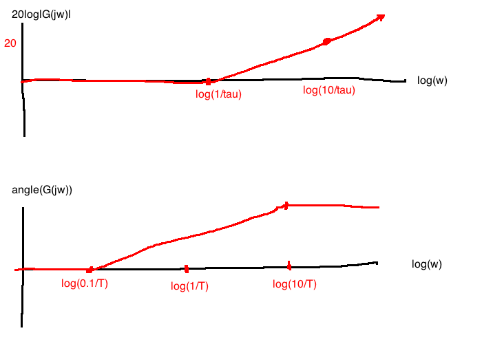
For \(G(j\omega)=j\tau \omega + 1\) (the transfer function with a zero at \(s=\frac{-1}{\tau}\))
Polar:
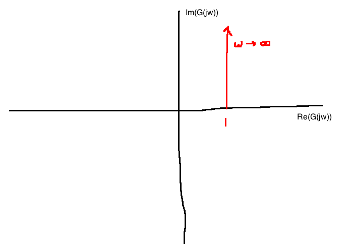
Bode:
Approximations for sketching:
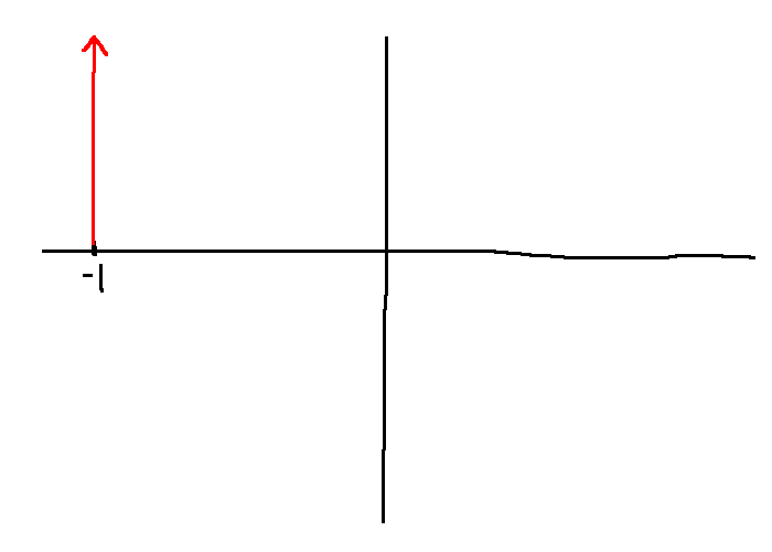
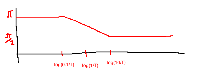
Sub-case: \(G(s) = \tau s - 1\) (zero at \(s=\frac{1}{\tau}\))
Polar plot:
e.g. \(G(s) = \frac{100}{s+10} = \frac{100}{10} \cdot \frac{1}{\frac{s}{10}+1} = 10 \frac{1}{\frac{s}{10}+1}\)
Frequency response: \(G(j\omega)=10\frac{1}{\frac{j\omega}{10}+1}\)
Magnitude: \(20\log|G(j\omega)|=\underbrace{20\log10}_{A}-\underbrace{20\log\left|\frac{j\omega}{10}+1\right|}_B\)
Phase: \(\angle G(j\omega) = \underbrace{\angle 10}_A - \underbrace{\angle \frac{j\omega}{10}+1}_B\)
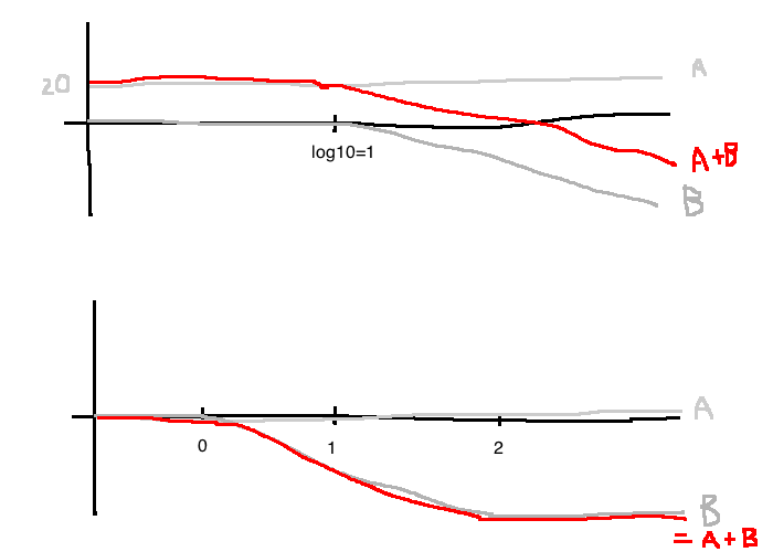
The bandwidth of the above system is the smallest frequency \(\omega_{BW}\) such that:
\[|G(j\omega_{BW})|=\frac{1}{\sqrt{2}}|G(0)|\]
In dB: \(20\log|G(0)|-20\log|G(j\omega)|=3dB\)
From the Bode plot, \(\omega_{BW}=1.0 \text{ rad/s}\)
e.g. \(G(s)=s^n\)


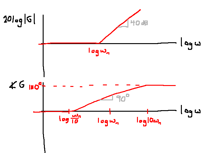
\[G(s) = \frac{s^2}{\omega_n^2}+\frac{2\zeta}{\omega_n}s + 1, \quad \zeta \in [0,1), \quad \omega_n \ne 0\]
\[G(j\omega)=\left(1-\frac{\omega^2}{\omega_n^2}\right) + j\cdot 2\zeta \frac{\omega}{\omega_n}\]
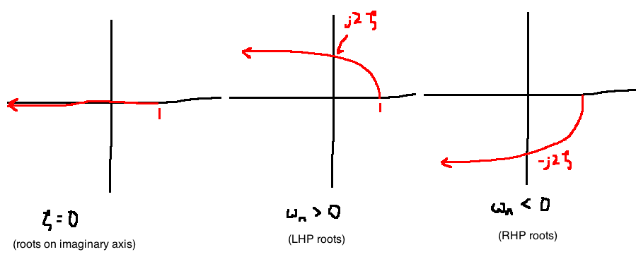
Observations:
For asymptotic Bode plots of complex conjugate roots, approximate \(G(s)\) as two first order terms with roots at \(-\omega_n\). i.e., set \(\zeta=1\):
\[\begin{align}
G(s)&=\frac{s^2}{\omega_n^2}+\frac{2\zeta s}{\omega_n} + 1\\
&\approx \frac{s^2}{\omega_n^2}+\frac{2s}{\omega_n}+1\\
&=\left(\frac{s}{\omega_n}+1\right)^2\\
&= (\tau s + 1)^2, \quad \tau = \frac{1}{\omega_n}\\
\end{align}\]
\[g(t) = Ce^{At} 1(t) + D \delta(t)\]
\[G(s) = C(sI-A)^{-1}B+D\]